
EBSILON®Professional Online Documentation


The components of EBSILON®Professional are originally based on physical equations that are valid in steady state. Transient or dynamic calculations are therefore not possible. Many components have therefore been extended accordingly so that transient calculations are also possible with them.
Examples are the behavior of plants over a certain period of time, for example over a day or over a year (solar power plants) or over a shorter period of time (start-up of a conventional power plant, charging/discharging of electric batteries).
If one wants to calculate dynamic processes, the time series calculation is to be used. The calculation is controlled by one of the tables, which can be opened with the menu "Calculate -->Time series".
The time series calculation enables the calculation of a sequence of calculations for a given time range. In order to use the time and location information (position of the sun, geographical position...), it may be necessary to have a component 117 "Sun" in such a model. Components that require such data have a default value ISUN, which is used to refer to a component 117.
The module "Time Series Calculation" was originally developed in connection with the EbsSolar module, but is used for all transient calculations. These are also those transient calculations where the time-dependent heat storage in fluids and components is considered.
The first available transient components were the storage components 118 and 119. In the meantime, many of the existing components have been extended so that they can be used to model the heat storage capacity of both the fluid quantities located in the component and the masses of the component itself. A current storage component "battery" and corresponding control components (PID) are also available.
These components can be found via Insert-->Component-->Instationary. If these components are to be used for transient calculations, additional information about the mass, heat or current storage capacity (geometry, materials, masses, nominal capacity) of the component must be provided.
Also, the nominal values of such a component cannot be left blank - even if the calculation is based on geometry data only. This is because, in the case of partial load in a sub-profile, it is possible to switch from a geometry-based calculation method to a non-geometry-based method (or vice versa).
The selection of the time discretization of the heat exchange calculation is defined with the default values FALGINST, FALG
(valid for components 9, 20, 119, 126, 160) :
The selection of the spatial discretization (numerical scheme) is defined with the default value FNUMSC (valid for components 7, 10, 126)
For components 7, 10, 61, 119, 126 and calculation with FALG=1 in component 124, you can use the FDPNUM switch to specify the calculation of the pressure drop for numerical calculation (FALG=1).
If FDPNUM = 0, an average value of the fluid pressure between inlet and outlet is used for the calculation.
If FDPNUM = 1, a linear pressure distribution between the inlet and outlet is assumed and the corresponding pressure values in the individual fluid elements (number controlled via NFLOW) are used for the calculation.
The calculation is controlled via tables that are activated with the menu "Calculate” à "Time series".
These tables are saved together with the model. Via the clipboard, cells from a table can also be exported to Excel and re-imported from Excel.
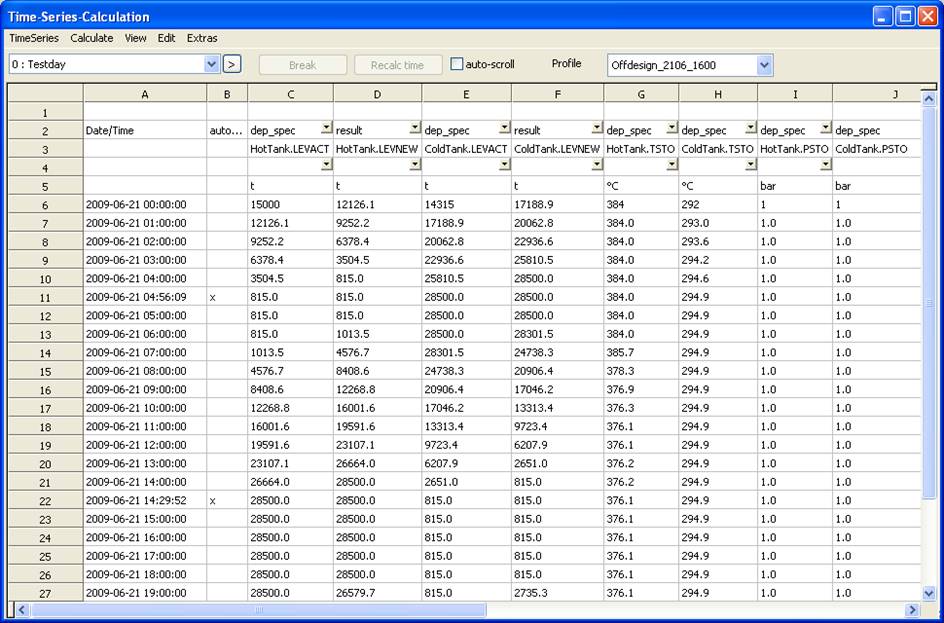
The table is structured as follows:
In column A, the points in time to be calculated are to be specified.
The interval between two points in time determines the change of the storages from one point in time to the next.
If, within such a period of time, one or more storage components reach their lower or upper limit, the time calculation will automatically split up the time range and insert an interline. These will be marked with an "x” in column B.
From column C on, values to be set or output at the respective point in time can be defined. There are three categories of values:
Before the calculation, the value is adopted into the model from the row to be computed.
Before the calculation, the value is copied automatically from the respective value of the previous timer series row into the time series row to be computed, and adopted into the model. In the case of the storage component 118 this is necessary for the following specification values:
A field (or characteristics) or a matrix can also be a time-dependent default value.
All time-dependent default values can be automatically inserted into a time series using the menu item "Edit --> Update headers --> For all components". The time-dependent value "transientstate" is then entered for each transient component. This one time-dependent value provides the component results of all time-dependent values of this component at the end of a time step as start values for the next time step.
Result value
After the calculation, the value is adopted from the model into the computed row. Terms can be specified as result value, too. These are then evaluated by EbsScript.
Line results represent average values of an interval (time step).
Component results are stored together with the components and represent values at the end of an interval (time step).
Row 1 is at freely available for headlines and remarks and is not evaluated by the program.
Row 2 contains the type and row 3 the name of the values or the term to be calculated.
In row 4, a processing of the result values by the time series module can be selected. There are the following options:
In row 5, the unit can be specified. If the field is empty, the respective standard unit will be used. The conversion can be effected in both directions, on the assumption that the value in the model is present in standard units, and the value in the table in the specified unit. The conversion also works for terms, since these are always evaluated in standard units by EbsScript.
From row 6 on, the data of the table follow. The calculation ends when an empty time specification is found in one row.
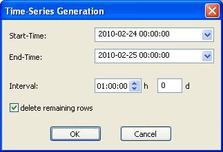
Several time series can be saved in one model. A new time series is generated under the menu "Time series” with the command "Add". With "Edit”, "Add headlines", standard values can be allocated to the headlines. In the process, the time-dependent values and the respective result values of all storage components are inserted into the table. With "Edit”, "Generate time stamp”, also the column with the points in time can be pre allocated. This is done by specifying a starting time and an end time and the desired time interval between two entries.
Time functions used in the time series calculation
@calcoptions.res.rtimemax:
(Specification value via time stamp generation: desired time interval between two time steps)
rtimemax is the remaining time the model can run in the current mode of operation. If this is not the case, because this time step is less than the specified interval between the time steps, an interval marked with “x“ (see column B) will be output and suitable measures for continuing the operating condition will be taken (e.g. alternating charging and discharging of the hot and cold storage system).
@calcoptions.res.rtime
rtime is the result value (storage component) representing the "remaining time" in which e.g. a storage component might be charged/discharged until the filling level reaches the MAX or MIN value.
By way of example, the sample model "Solarfield_GeoModel.ebs" contains two annual data records of the sites Usak (Turkey) and Sarroca de Lleida (Spain), kindly provided by the company Geomodel (www.geomodel.eu). If required, you can also receive data on weather and insolation for other sites there.
After creating the table, it is advisable to first activate Check input under the menu item "Calculate" in order to be made aware of possible syntax errors. Likewise under the menu item "Calculate”, the calculation is then started. Here, optionally everything or only the selected rows or the row up to the selection or starting from the selection or also only one single row can be computed.
In the "Auto Scroll" mode, the rows are moved up in the process so you can watch the course of the calculation.
After the calculation, the results are contained in the table. It is also possible to display them in a diagram (under the menu item "Extras" ).
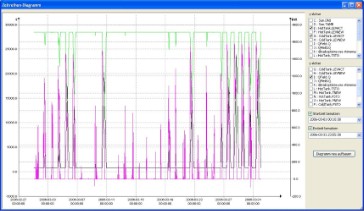
Image Title
In the diagrams, the time is plotted on the x-axis; the period of time can be chosen or adopted from the table. The quantities to be represented can be selected and distributed to two y-axes.
Note:
Displaying diagrams while using the time series dialog
By default, values of the time stamps shown on x-axis can cause incorrect plots of calculation results. If there are to be non equidistant intervals in time series, discontinuities in curves may occur, though the results don’t have any steps or jumps.
Example of time series dialog:
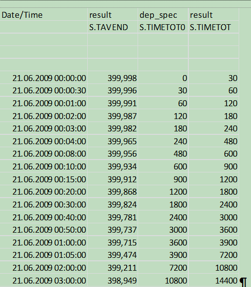
The result values “S.TAVEND” don’t really start at point t0 (first time step), but with the step t1. In fact, that means the line containing the time step t shows already the result of the calculation t+dt. Here, the line “21.06.2009 00:00:00“ holds the values of „21.06.2009 00:00:30“. While equidistant steps provide only a shift on x-axis, non equidistant time steps lead to wrong pairing. In these cases it´s necessary to choose the option “A: Date/Time (at end) for displaying the x-axis. For further needs there´s also an option to select “A: Date/Time (at median)”, e.g. the average between two time stamps.
There is an interface unit "Timeseries" by means of which you can access the time series calculation from EbsScript.
In the time series, you can enter commands in the field B4 to execute an EbsScript and to select a profile where the calculation is to take place. The syntax for this is:
ebsscript:"EbsScript-Name";profile:Profile-Id